Week 7 - OpenAI Project

Natural Policy Gradients, TRPO, A2C

Most of the recent successes in reinforcement learning comes from applying a more sophisticated optimization problem to policy gradients. This week I learned about advanced policy gradient techniques using algorithms such as Natural Policy Gradients, TRPO, and A2C.

I implemented Lab 4 provided by the Deep RL Bootcamp [1] [3]. My code is here [GitHub Source]

Standard Policy Gradient Algorithm

I had already done some training of Atari’s Pong during Week 4 with policy gradients and Tensorflow. In Lab 4, we made the gradient calculations manually.

Gradient Calculation for One Timestep

R_t = (discount * R_tplus1) + r_t
grad_t = get_grad_logp_action(theta, s_t, a_t) * (R_t -b_t)

Accumulate Gradient Across Timesteps

grad += grad_t

Update Parameters

theta += learning_rate * grad

Natural Policy Gradient

Natural Policy Gradient improves on the standard policy gradient algorithm by approximating an optimization problem using a Fisher Information Matrix and step size.

Compute KL-divergence Hessian/Fisher Information Matrix

Take the parameters (theta) and calculate the gradient for an observation and action pair. Add the gradient values to a matrix.

d = len(theta.flatten())
F = np.zeros((d, d))
for ob, action in zip(all_observations, all_actions):
	grad_logp = get_grad_logp_action(theta, ob, action).flatten()
	F += np.outer(grad_logp, grad_logp)
F /= len(all_actions)

Compute Natural Gradient

Take the Fisher Information Matrix (F) from above and add small values (reg) along the diagonal to ensure it’s a positive definite, then invert it. Multiply the F_inv with the policy gradient.

F_inv = np.linalg.inv(F + reg * np.eye(F.shape[0]))
natural_grad = F_inv.dot(grad.flatten())

Compute Step Size

Using the second order approximation to the KL divergence, compute the adaptive step size using the natural gradient (natural_grad), the Fisher Information Matrix (F), and natural_step_size.

g_nat = natural_grad.flatten()
step_size = np.sqrt((2 * natural_step_size) / (g_nat.T.dot(F.dot(g_nat))))

Update Parameters

theta += step_size * natural_grad

Advanced Policy Gradients

When calculating the surrogate loss, the gradient can be made more invariant by averaging over time steps in different trajectories. The distribution parameters (dists) are calculated using a flattened list of observations across all trajectories in a batch.

Surrogate loss is computed by taking the log likelihood or probability of the actions (all_acts) under the distribution parameters (dists). Multiply this value with the estimated advantages (all_advs) and take the negative mean.

Surrogate Loss for Policy Gradient

surr_loss = -F.mean(dists.logli(all_acts) * all_advs)

Trust Region Policy Optimization (TRPO)

TRPO [4] uses a constraint on the KL divergence. The region defined by this constraint is called the trust region. In addition, it computes the approximate natural gradient using conjugate gradient.

Surrogate Loss for TRPO

TRPO modifies the Surrogate Loss calculation to calculate the likelihood ratio between the old and new distribution parameters before multiplying it with the estimated advantages and taking the negative mean:

likelihoods = new_dists.likelihood_ratio(old_dists, all_acts)
loss =  -F.mean(likelihoods * all_advs)

KL Divergence

Calculate the average KL divergence between the old and new distribution parameters.

kl = F.mean(old_dists.kl_div(new_dists))

(Synchronous) Advantage Actor-Critic (A2C)

Combines Policy Gradients and Deep Q Learning using two networks, the actor and critic. The Actor network takes the observation and outputs the best action in a continuous space. The Critic takes the observation and actor’s action as inputs and predicting Q values. The Actor will move in the direction of suggested by the Critic.

Compute Returns and Advantages

Start at time step t and use future_rewards to calculate empirical returns and advantages.

returns = np.zeros([rewards.shape[0] + 1, rewards.shape[1]])
returns[-1, :] = next_values
for t in reversed(range(rewards.shape[0])):
future_rewards = discount * returns[t + 1, :] * (1 - dones[t, :])
returns[t, :] = rewards[t, :] + future_rewards
returns = returns[:-1, :]
advs = returns - values

Total Loss for A2C

Use the surrogate loss implementation from standard policy gradient, but add an entropy bonus with coefficient ent_coeff. When calculating total_loss, use the coefficient vf_loss_coeff with the value function loss from the Critic.

policy_loss = -F.mean(logli * all_advs + ent_coeff *  ent)
vf_loss = F.mean(F.square(all_returns - all_values))
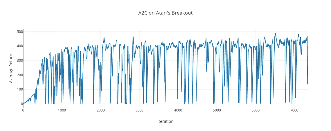
total_loss = policy_loss + vf_loss * vf_loss_coeff

A2C on Breakout

Here is the Average Rewards after training A2C on Atari’s Breakout:

Trained Policy Playing Breakout:

References

1. John Schulman. “Deep RL Bootcamp Core Lecture 5 Natural Policy Gradients, TRPO, and PPO”. Video | Slides
2. Sergey Levine. “CS294 Learning policies by imitating optimal controllers”. Video | Slides
3. Deep RL Bootcamp Lab 4: Policy Optimization Algorithms. Website
4. John Schulman et al. “Trust Region Policy Optimization”. PDF.
5. Dimitri P. Bertsekas. “Dynamic Programming and Optimal Control” Website.